Finally, two and a half after the beginning of GSoC 2021, we are almost ready to wrap up! Last week we introduced some important changes to our code, refactoring the way GridapMakie.jl calls the plotting functions. We were able to extend Makie’s plot, mesh, wireframe and scatter to adapt them to Gridap’s types ::Grid, ::Triangulation and ::CellField. In this post I will show some results, all of them extracted from the README in GridapMakie.jl. There you will find additional information as well as a list of examples to be reproduced in your own computer! In addition to that, this Pull Request will contain a description of the project, which shall be provided to Google as the final evaluation report.

Let’s get to some results! Since in this post we already saw some grid plots, we may as well try other things. For example, we can plot functions defined on the cells of a 2D triangulation:

or a function defined on the nodes of the boundary of such triangulation:

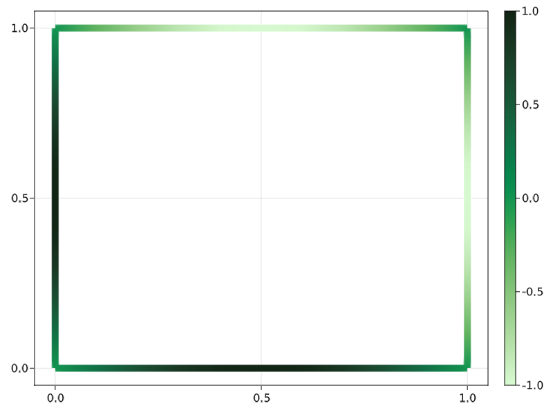
Again, all the commands needed to plot these figures along a thorough description can be found on the README file.

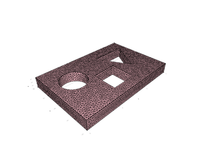
However, what we really want to see are the capabilities of GridapMakie.jl when having to plot more complex geometries. Let us take the geometry considered in the first Gridap tutorial, so that we can plot it with the edges of the cells on the boundary:

At this point, we may be convinced that GridapMakie.jl has been worth the effort and will prove to be quite useful and comfortable to all users, but that’s not all! The package hides an ace up on its sleeve, since it can make use of Makie’s interactivity and create observables that can be updated in real time. For example, we can record animations:

Overall, even though it has many limitations, GridapMakie.jl steps up to be a clear alternative to using external software such as Paraview.