After a period of getting to know Makie and trying to find the best approach for Gridap grids, we came up with a suitable way of plotting simplexified (i.e. made up by triangles) grids.

Moreover, not only did we implement the recipes faces and edges but also vertices, letting us plot something like

using Gridap, GridapMakie, GLMakie

# Create our square grid made up by triangles (or elements):
model = CartesianDiscreteModel((0,1,0,1),(5,5)) |> simplexify
grid = get_grid(model)

# Plot faces, edges and vertices:
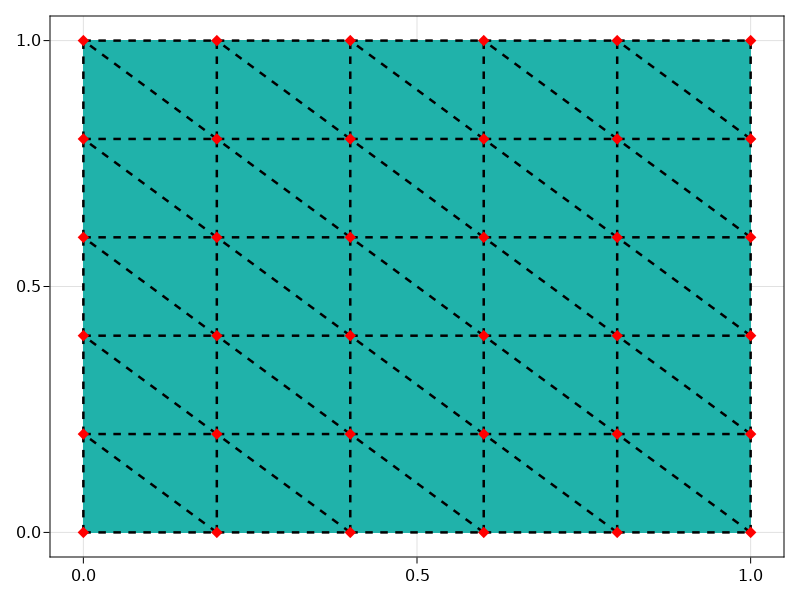
fig = faces(grid, color=:lightseagreen, shading=true)
edges!(grid, color=:black, linestyle=:dash, linewidth=2.5)
vertices!(grid, color=:red, marker=:diamond, markersize=15)
fig

which will return the following figure

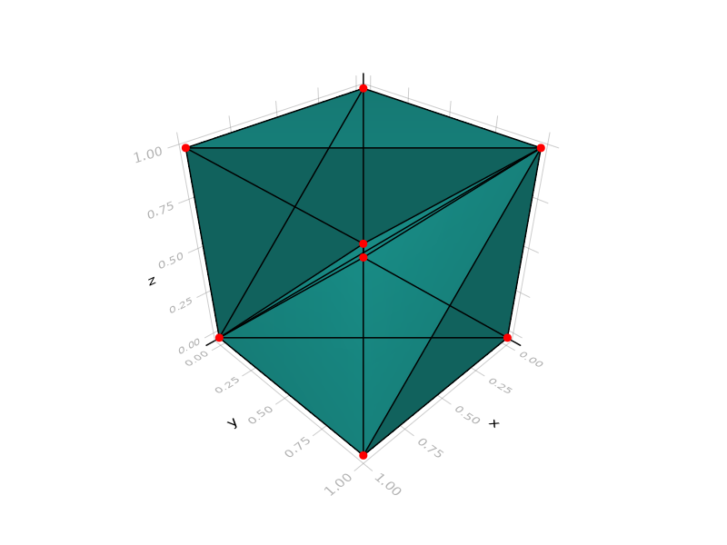
We note here that faces returns a tuple of objects, those being a Figure and an Axis. By making use of the former, we may plot several objects on top of each other, for example lines and dots over a painted surface. Such behaviour can be extended to 3D, like

# Create our square grid made up by triangles (or elements):
model = CartesianDiscreteModel((0,1,0,1,0,1),(1,1,1)) |> simplexify
grid = get_grid(model)

# Plot faces, edges and vertices:
fig = faces(grid, color=:lightseagreen, shading=true)
edges!(grid, color=:black)
vertices!(grid, color=:red)
fig

resulting in

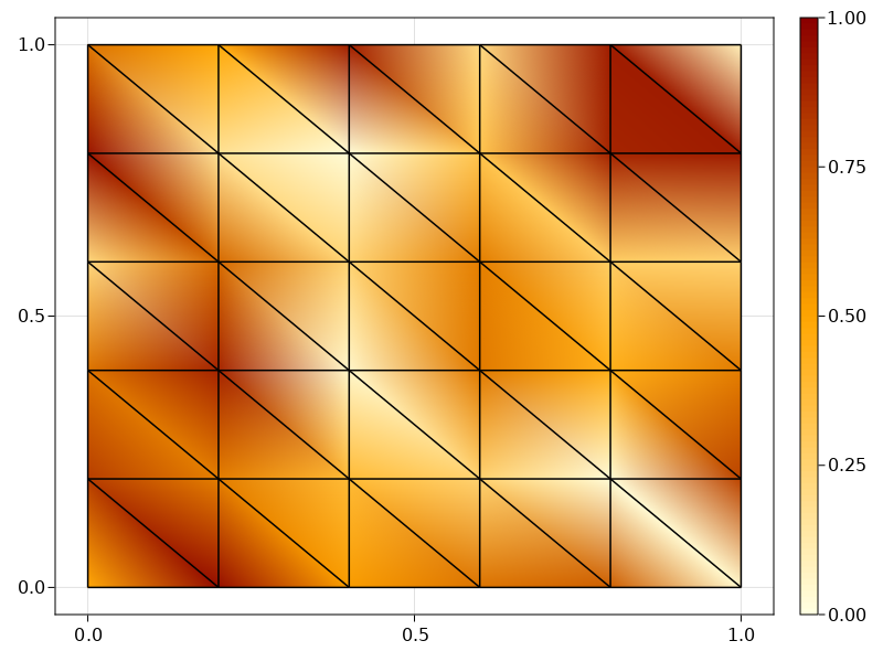
Even though we already have implemented the use of colors to represent scalar nodal or cell fields, they are limited to simple arrays, e.g. nodaldata = rand(num_nodes(grid)) in (note the use of a colorbar)

fig, _ , plt = faces(grid, color=nodaldata, colormap=:heat, colorrange=(0,1))
edges!(grid, color=:black)
Colorbar(fig[1,2], plt, ticks=0:0.25:1)
fig

seen as

Therefore, our next step is to adapt the solution representation to Gridap types.